Statistical inference (or inferential statistics) is the procedure by which the characteristics of a population are induced by the observation of a part of it (called “sample”), usually selected through a random (random) experiment. From a philosophical point of view, these are mathematical techniques to quantify the learning process through experience.
We will mainly consider simple random samples of size n> 1, which can be interpreted as n independent realizations of a basic experiment, under the same conditions. Since a random experiment is considered, the probability calculation is involved.
Example:
Given an urn with a known composition of 6 white balls and 4 red balls, using the rules of the probability calculation we can deduce that if we extract a random ball from the urn, the probability that it is red is 0.4. Instead we have a problem of statistical inference when we have an urn whose composition we do not know, we extract n balls at random, we observe its color and, starting from this, we try to infer the composition of the urn.
In the field of statistical inference, we distinguish two schools of thought, linked to different conceptions, or interpretations, of the meaning of probability:
– Classical or frequentist inference;
– Bayesian inference.
Bayesian inference is therefore just the process of deducing properties about a population or probability distribution from data using Bayes’ theorem. That’s it.
Bayes’s Theorem:
Before introducing Bayesian inference, it is necessary to understand Bayes’ theorem. Bayes’ theorem is really cool. What makes it useful is that it allows us to use some knowledge or belief that we already have (commonly known as the prior) to help us calculate the probability of a related event.
Mathematically Bayes’ theorem is defined as:

where A and B are events, P(A|B) is the conditional probability that event A occurs given that event B has already occurred (P(B|A) has the same meaning but with the roles of A and B reversed) and P(A) and P(B) are the marginal probabilities of event A and event B occurring respectively.
The Bayesian view of probability is related to degree of belief. It is a measure of the plausibility of an event given incomplete knowledge.
Decision makers use their beliefs to construct probabilities. They believe that certain values are more believable than others based on the data and our prior knowledge.
The Bayesian constructs a credible interval centered near the sample mean and totally affected by the prior beliefs about the mean. The Bayesian can therefore make statements about the population mean by using the probabilities.
Bayesian inference is an extremely powerful set of tools for modeling any random variable, such as the value of a probability of a diagnose, a demographic statistic. We provide our understanding of a problem and some data, and in return get a quantitative measure of how certain we are of a particular fact. This approach to modeling uncertainty is particularly useful when:
- Data is limited
- We’re worried about overfitting
- We have reason to believe that some facts are more likely than others, but that information is not contained in the data we model on
- We’re interested in precisely knowing how likely certain facts are, as opposed to just picking the most likely fact
Typically, Bayesian inference is a term used as a counterpart to frequentist inference. This can be confusing, as the lines drawn between the two approaches are blurry. The true Bayesian and frequentist distinction is that of philosophical differences between how people interpret what probability is. We’ll focus on Bayesian concepts that are foreign to traditional frequentist approaches and are actually used in applied work, specifically the prior and posterior distributions.
Consider Bayes’ theorem (C=Cause and E=Effect):
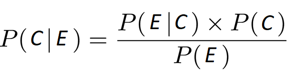
where P(C|E) is called a posteriori probability and P(C) is the a priori probability and P(E|C) is the likehood and P(E) is the normalization factor.
Think of C as some proposition about the world, and E as some data or evidence. For example, C represents the proposition that it rained today, and E represents the evidence that the sidewalk outside is wet:
P(C=rain | E=wet) asks, “What is the probability that it rained given that it is wet outside?”
To evaluate this question, let’s walk through the right side of the equation. Before looking at the ground, what is the probability that it rained, P(rain)? Think of this as the plausibility of an assumption about the world. We then ask how likely the observation that it is wet outside is under that assumption, P(wet | rain)? This procedure effectively updates our initial beliefs about a proposition with some observation, yielding a final measure of the plausibility of rain, given the evidence.
This procedure is the basis for Bayesian inference, where our initial beliefs are represented by the prior distribution P(rain), and our final beliefs are represented by the posterior distribution P(rain | wet). The denominator simply asks, “What is the total plausibility of the evidence?”, whereby we have to consider all assumptions to ensure that the posterior is a proper probability distribution.
Bayesians are uncertain about what is true, and use data as evidence that certain facts are more likely than others. Prior distributions reflect our beliefs before seeing any data, and posterior distributions reflect our beliefs after we have considered all the evidence.
